
|
|
|
|
2018年12月02日 |
|
|
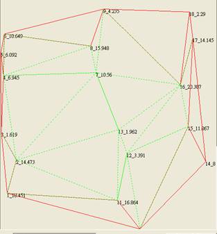
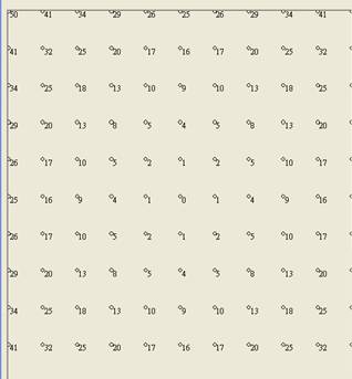
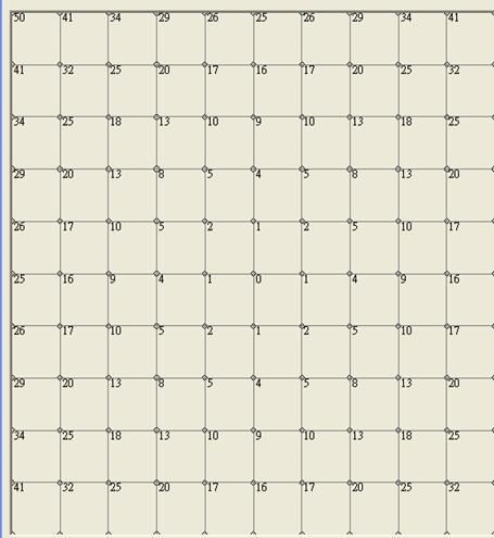
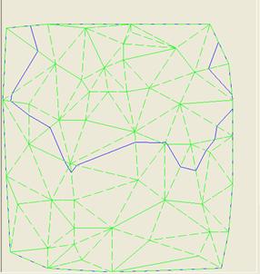
Contour Graphs in VB Contour line surface are surface lines with same elevation (z value) in three dimensional spaces (3D), and 2D contour lines are projection drawing of 3D contour on z plane. Contour map lines can be symbolized by different colors or levels of gray scale, labeled contour lines, or both. In Cartesian space, plotting a contour map can be summarized as following six steps: (1) Data input (2) Creating triangles (or rectangular grid) (3) Liner interpolation (4) Drawing of contour line segments (5) Connecting, smoothing (6) Coloring and labeling Data input In general, the control points of topography contour line are located without any particular regularity while some contour function[z=f(x,y)], or two variables parametrical function [x=f(u,v),y=g(u,v),z=h(u,v)] are regularity. For scatter data we can use triangle algorithm to plot the contour, or we convert scatter data to regular spaces grid data by interpolation and then use Rectangle algorithm to plot the contour. Creating triangles or rectangular grid cells All data can be connected to create Delaunay (Thiessen) triangles in x_y plane. It is obvious that the control points can be connected in different manner. Generally, different sets of triangulations will get different result. To avoid this problem, the best way of connecting triangles seem to select a unique and optimal set of triangles, it is mean that the individual triangles should be as near to equilateral as possible. Among the algorithm of triangulations, the so called Delaunay triangulation (Figure 1), are uniquely defined for a given set of points and triangles with nearly equiangular as possible. For some mathematical function, the data points are spaced regular on a grid or network (Figure 2).
Figure 1
Figure 2
Linear interpolation (a)Linear interpolation of Delaunay triangle To find the intersection of a contour line with a given level zg and one side of a Delaunay triangle with coordinates (xi,yi,zi) and (xj,yj,zj) , we can compare the zmin and zmax values of each triangle, if zg value is lay above zmax or below zmin, it means that the contour line with level zg do not intersect this triangle, then we can neglect these triangles, if zg value is between zmin and zmax, it means that this contour line will intersect two sides of this triangle, we can calculate the (x,y) coordinate of the line segment of each triangle as following: ‘---------------------------------------- If abs(zi-zg)* <eps and abs(zj-zg)* <eps then LineSeg.pt1.x = xi ‘lineSeg =Line segment of contour LineSeg.pt1.y = yi LineSeg.pt2.x = xj LineSeg.pt2.y = yj End if ‘----------------------------------------- If abs(zj-zg)* <eps then xg = xj yg = yj End if ‘------------------------------------ If abs(zi-zg)* <eps then xg = xi yg = yi End if ‘-------------------------------- If abs(zj-zg)* <eps then xg = xj yg = yj End if ‘------------------------------------- If (zi-zg)*(zj-zg) <0 then xg = xi + (xj - xi) / (zj - zi) * (zg - zi) yg = yi + (yj - yi) / (zj - zi) * (zg - zi) End If ‘-----------------------
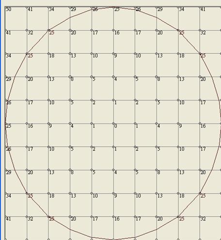
Figure 3 (b)Linear interpolation of Grid cell A scatter data can be converted to regular space data (Figure 4). Suppose the four nearest scatter data with distance a, b, c, d to the estimating point, and given z values za, zb, zc, zd, respectively, then the z value (zans) of concerned grid point can be calculated as: zans=(za/a+zb/b+zc/c+zd/d)*(1.0/a+1.0/b+1.0/c+1.0/d)
Figure 5 The implement of interpolation of a contour line with given value and a rectangular grid was introduced by Paul Bourke, Byte in June 1987, The rectangular grid is considered four points at a time, namely the rectangle A[x(i),y(j)], B[x(i+1),y(j)], C[x(i),y(j+1)], and D[x(i+1),y(j+1)]. The centre of each rectangle (Figure 6) is assigned a value corresponding to the average values of each of the four vertices. Each rectangle is in turn divided into four triangular regions by cutting across two diagonals. Each of these triangular planes may be bisected by a horizontal contour plane. The intersection of these two planes is a straight line segment (parts of the contour curve for a given contour level).
Figure 6 Depending on the value of a contour level with respect to the height at the vertices of a triangle, certain types of contour lines are drawn. The 10 possible cases (Figure 7) which may occur are summarized below:
(a) All the vertices lie below the contour level
(no intersection). In cases a, b, i and j two planes do not intersect, ie. no line need be drawn. For cases d and h the two planes intersect along an edge of the triangle and therefore line is drawn between the two vertices that lie on the contour level. Case e requires that a line be drawn from the vertex on the contour level to a vertex on the opposite edge. This point is determined by the intersection of the contour level with the straight line between the other two vertices. Case c and f are the most common cases where the line is drawn from one edge to another edge of the triangle. The last possibility or case g has no really satisfactory solution, it
fortunately will occur rarely with real arithmetic.
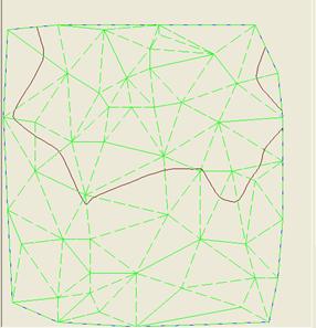
Drawing of contour line segments Suppose we want to plot the contour with nLvel(no of line level)=10, and z value from z1 to z2. Then we start from some specific zg=z1 by tracing from the first triangle to compare zg with the zmin and zmax values of each triangle, if zg value is between zmin and zmax, then we calculate the line segment across this triangle (Figure 8). The tracing must go from one triangle to another triangle until all the triangles have been finished.
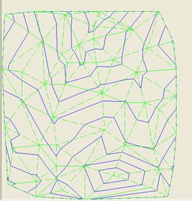
Figure 8 Following same procedure, we trace another loop with zg= (z1+dz), …..until zg>=z2. Connecting and smoothing The locations of line segments for every zg value are irregular distributed ( Figure 9), so we need to joint the line segments to a polyline (or polylines), in order to smooth them. To smooth each polyline we can use Bezier or Spline curve (Figure 10) to substitute in VB 6.0,while in Vb.Net we can use Drawcurve or DrawClosedCurve methods to smooth the contour lines.
Figure 9
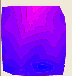
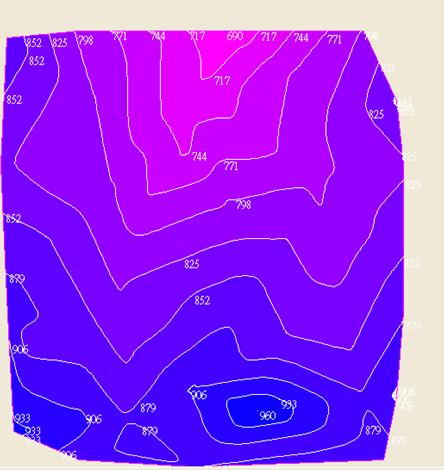
Figure 10 Coloring and labeling To fill the color between two consecutive contours, you need to draw the outbound polyline of the map first, and then (1) To flood fill the outer region of contour map first with the color similar but different to the back color of the PictureBox (zone 1 in Figure 11). (2) To flood fill the closed contour line with Api function polygon(zone 2 in Figure 11) in VB 6 or FillPolygon in VB.NET. (3) Walking along the outer boundary line (ABCDEFGHI, Figure 11) ,To connect the outer control point(A~E) and point (Cen, center of pictureBox), and select a point M ,where the pixel color same as backcolor of picturebox, to be a seed point of flood fill and to color the zone(Zone 3) with Api ExtFloodFill function both in VB 6 and Vb,net to fill the zone between two consequence contour lines. To label a contour is quite simple and easy, you can label it near the beginning and ending of a contour line, or simple near the center of a closed contour.
Figure 11
Figure 11
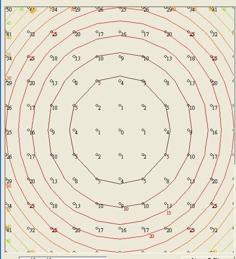
Figure 12 Something about Function ConRec Function ConRec was introduced (Fortran language) by Paul Bourke, Byte in June 1987, which can use to plot contour of regular grid data. Figure 13 is the result by using the modified Function ConRec in VB 6.0 without smoothing.
Figure 13
|
上次修改此網站的日期: 2018年12月02日